Vignetting Revisited

After enduring a little confusion and frustration in correcting some images from my Canon G9 camera, I investigated a little more and found that my process needs to be changed. A while back, in Part 2: Vignette Correction, I described a way to mathematically characterize and correct image vignetting. It was fine theoretically but, in practice, I found a little surprise.

To get a better idea of the vignetting characteristics, and not having a proper optical opal glass, I improvised using some nice polyester drafting film I had laying around. I cut 2 pieces and sandwiched them between cardboard mats to create a nice white diffuse window about 3 inches in diameter. I aim the camera up at a dull gray overcast sky, place the diffuser on top of the lens hood, and shoot at the various apertures. This worked pretty well for a quick test.


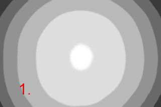
Image 1 is an example of a shot using this technique with some post-processing to really draw out the shape of the light falloff. (In Photoshop I posterized the image and boosted the contrast.) This particular shot was using a 24 mm lens at f/2.8 on a Nikon D700 dSLR. It shows the expected radial light fall-off. It is this shape of light falloff that responds well to the mathematical corrections I described earlier. Also vignette tools in Photoshop and other image editors would handle this fairly easily if not quite as precisely.


So, what's the problem with the G9? Take a look at image 2 which was shot with the G9 at 7.4mm focal length (the shortest of the zoom range) at f/2.8. It was processed in a manner similar to the other one to draw out the tonal structure. You can see the problems: the brightest part is not in the center of the image, there is less of the well-behaved radial symmetry seen in the first image, and the shape doesn't resemble the neat bullseye we saw earlier.

Sampling readings in various parts of the image show that each corner has a different tonal value (unlike the better-behaved first image). The lightest corner is more than 12% lighter than the darkest corner. These asymmetries make it impossible to use the mathematical technique, based on radial symmetry, that I was trying to use up to this point, at least not with best results.

The solution is to use this flatfield image (without the adjustments used for illustrative purposes) as an adjustment template to precisely match tonal corrections to actual system characteristics. A tool like the fulla command discussed extensively in earlier posts handles this nicely:

 fulla -f flatfield_image target_image

We simply use a flatfield image shot at the same focal length and aperture as the target image and fulla will apply corrections to compensate for the vignetting characteristics no matter how odd they may be. Of course now this means that you need flatfield images for each of the focal length and aperture combinations you use. As I've mentioned earlier, this is a bit simpler for the G9 in that I only use f/4 or f/5.6, the sweet spot between lateral chromatic aberration and diffraction limits.

At this point, I've ordered some opal glass (not expensive) so I can do more careful flatfield images to get optimal corrections of vignetting.

So, what's the deal with the odd G9 characteristics? I don't know really. Based on this sample of one camera, I'm guessing that there are manufacturing variations and less-than-perfect alignment in the system but there are other possibilities in the engineering of the system that may help explain the odd behavior. By the way, the off-center vignetting asymmetry moves and changes shape slightly as you go through the zoom range. Go figure. I'll bet these kinds of variations are common in the compact and consumer class of cameras in general.

I have enough of a grasp on reality to know that this level of fussing is way beyond what most people feel there's a need for. Frankly I haven't lost a great deal of sleep over it either but it's fun to try to squeeze out the best images you can from what you're working with.

Part 5: Putting It All Together

In previous posts, we've looked at the Canon G9 point-and-shoot camera's vignetting, geometric distortion, and chromatic aberration. We've also looked at strategies for addressing these issues, primarily using the fulla command from the hugin panorama photo stitcher package.

The fulla command doesn't have a nice friendly GUI interface but it does allow us to put together arbitrary corrections to be applied to large numbers of images without a great deal of effort. Each of the fulla corrections we've explored in previous posts can be combined into a single command addressing vignetting, geometric distortion, and chromatic aberration.

Your workflow sequence is very important. The corrections we've been discussing should be applied to the images before any cropping, resizing, etc. have been done. I always shoot raw so I use ACR or some other tool for "developing" the image to set the correct initial tonality, color temperature, etc. and then export the image in 16-bit TIFF format (lossless unlike JPEG). I apply the image corrections and then bring the corrected version into Photoshop for subsequent processing.

Let's start with a hypothetical file shot on the Canon G9 at 7.4 mm and f/4, and processed from the raw CR2 file into a 16-bit TIFF file called example.tif. To apply my standard corrections for vignetting, geometric distortion, and chromatic aberration, I would use the following command:

fulla -c 1.0398:-0.1155:0.1954:-0.1605 \ 
      -g 0.028:-0.0871:0.0521:1.007 \
      -r 0:0:0:1.00024 -b 0:0:0:1.00041 example.tif

(The '\' characters indicate arbitrary line breaks for formatting here. This is actually all one command line.)

The "-c" option gives the polynomial coefficients for correcting vignetting, the "-g" option gives the polynomial coefficients for geometric distortion correction, and the "-r" and "-b" options provided the polynomial coefficients for transverse chromatic aberration correction. (But you already knew that.)

When fulla is done crunching the numbers, it outputs a file with a "_corr" filename suffix. So our example correction would create a new file called example_corr.tif. It will look substantially better than the original with the corrections applied.

Naturally you don't want to have to type in that command every time you process a file so you can create a MSDos batch command file (on Windows) or a Bash script (on Unix systems) to generalize it. Let's say we want to correct arbitrary numbers of files with one command. We can create a batch file like this:

for %%f in (%1) do \
       fulla -c 1.0398:-0.1155:0.1954:-0.1605 \ 
      -g 0.028:-0.0871:0.0521:1.007 \
      -r 0:0:0:1.00024 -b 0:0:0:1.00041 %%f

(Once again, this should be all on one line in the real batch file.) Assuming you named this something like G9_74_4.bat (because it's only useful for the G9's 7.4 mm f/4 images), you can process all the TIFF files in a directory with a single command:

g9_74_4 *.tif

Unix, Linux, Mac users can create analogous script files using for iterations to do precisely the same thing.

I must mention something about the fulla command here: it's flaky and not mature in some regards. One frustration is that, when it outputs a corrected image, that corrected image has its metadata stored in an unconventional way that is not visible to Photoshop and many other applications. If you're running any kind of responsible workflow, this is not good, but there is a way around the problem.

ExifTool by Phil Harvey is a superbly-done high-function image metadata management tool. It has an extraordinary number of capabilities and it handles them well. If you download the tool, you can use it to save your EXIF (and other metadata) from your image, apply your fulla corrections, and then restore the original metadata in standard format. For example, you can save the metadata for all TIFF files in a subdirectory with this command:

exiftool -o %f.mie -ext tif .

Process your files using the fulla corrections and then restore the metadata to the corrected files.

exiftool -overwrite_original -tagsfromfile %-.5f.mie \
                       -ext tif .

You can even skip the intial save to MIE file (Meta Information Encapsulation) and simply rewrite the original file's metadata over the fulla output file:

exiftool -overwrite_original -tagsfromfile %-.5f.%e \ 
                       example_corr.tif

Finally, if you're really ambitious and have Perl programming skills, you could use the Perl Image::ExifTool package to determine the focal length and f-stop for the image and then do a table lookup to determine which of the fulla option parameters to use. I've done a rudimentary job of this just for the subset of camera settings I almost always use for the Canon G9.

If all these seems like a lot of trouble to correct the occasional image, you're right. It's most worthwhile if you routinely have large numbers of images you wish to optimize; then the use of fulla in batch or script files makes more sense.

If you only do occasional corrections, want something a bit easier to deal with, or want a commercial solution, stay tuned. Next up we'll glance at a couple of alternatives for correcting images that don't require all the up-front work we've been slogging through here.

Part 4: Chromatic Aberration

There are many reasons why an image may contain chromatic aberrations, the unexpected color casts or fringes in certain parts of the image. Lenses, particularly inexpensive ones such as found in point-and-shoot cameras, can contribute two main types of chromatic aberration: longitudinal (or axial) and transverse (or lateral).

Longitudinal chromatic aberration is caused by the lens system's failure to focus all wavelengths of light to the same focal plane. If we look, up close, at a piece of an image with sharp high-contrast edges, we can see evidence of longitudinal chromatic aberration in the unnatural blue and purple casts of leaves and branches in this example. This is part of a Canon G9 image shot at 7.4 mm at f/2.8.



The solution to longitudinal chromatic aberration is often quite simple: stop the aperture down, causing a greater overall depth of field and reducing the effect of the wavelength focus differences. When we close the aperture down to f/5.6, we notice a much better color rendition on this same subject.



From a series of tests on this subject, I notice the longitudinal chromatic aberration is mostly gone at f/4, and almost totally gone at f/5.6. There is no noticeable improvement if you stop down further. However, due to diffraction limitations, the image turns to mush, particularly at f/8. So, the rule of thumb is to stick between f/4 and f/5.6 to limit longitudinal chromatic aberration in images.

Transverse chromatic aberration is caused by the lens system enlarging the image on the focal plane to differing amounts depending on the wavelength of light. The effect is more noticeable the farther from the center of the image you look.

To evaluate transverse chromatic aberration, I taped a large (6 feet by 10 feet) sheet of white paper to the side of the garage and placed black electrical-tape X's all over it. This provided a target with a few handy properties for this exercise: relatively neutral tones (not favoring a particular color strongly), high contrast sharp edges between the black tape and white paper, and daylight illumination covering the whole visible spectrum (unlike, for example, fluorescent lights which have spikes at various wavelengths).



I set the Canon G9 camera to aperture-preferred f/4, framed the target to get useful X's to the corners, and shot at several focal lengths from the shortest, 7.4 mm, to the longest, 44.4 mm.

If we take a close look at the upper left corner of the 7.4 mm shot, we can see evidence of significant chromatic aberration around the X. (This sample of the full image is blown up to twice size and the saturation boosted way up to make the color aberrations quite clear.)

To correct this, we're going to use the fulla command mentioned frequently in previous posts. It's part of the freely-available hugin panorama photo stitcher package. The approach taken by the fulla command is to leave the green channel of the image alone and adjust the blue and red channels to line up correctly with the green channel. This makes a lot of sense since green appears brightest to our eyesight, there are twice as many green photo sites on a Bayer matrix sensor as there are either red or blue photo sites, and usually the green channel is the cleanest compared to the other two. Like we've seen in the discussions of vignetting and geometric distortion, fulla uses a polynomial to accurately represent adjustments to be made to each of the red and blue channels depending on radial distance from the center of the image. The polynomial adjustment, once again is of the form

 a * r3 + b * r2 + c * r + d 

There are a few ways we can approach finding the values for a, b, c, and d to use for correction. First, we can break the image into separate R, G, and B channel images and use one of the panorama stitching programs to compare the red and green channel images, select control points, and optimize the corrections for the red channel image required to make it line up with the green channel. Do the same thing comparing the blue channel image with the green channel, and we can get the set of polynomial coefficients that will shape the red and blue channels to line up with the green.

To break an image into separate channels, you can use Photoshop, go to the Channels tab, and select Split Channels. This will create 3 grayscale images, one for each color channel, with "_R", "_G", or "_B" appended to the filename to indicate which color channel it represents.

Another alternative to the tedium of fitting control points in a panorama stitching tool, is to use the tca_correct tool supplied in the hugin package. This command-line program also needs the separate channels broken out into separate image files with each beginning with "red_", "green_", or "blue_" denoting the channel it represents. An additional requirement is that each of the channel images must be an RGB image, not grayscale so that additional step would need to be done in Photoshop if you're going that route.

Another way to get the separate channel images broken out is through the use of ImageMagick a wonderfully powerful set of command-line tools available on all major platforms. Using ImageMagick's convert command we can extract each of the RGB channels into separate RGB image files:

convert %1 -channel R -separate -depth 8 -type TrueColor red_%1
convert %1 -channel G -separate -depth 8 -type TrueColor green_%1
convert %1 -channel B -separate -depth 8 -type TrueColor blue_%1

(This example uses a MSDos batch command file for Windows; the analogous thing can be done with the same parameters on the other platforms.)

The tca_correct command to evaluate your image and determine the polynomial coefficients is

tca_correct -o abc filename

where filename is the root file name without the color prefixes. After crunching things for a bit, it will show the fulla options to be used to correct the transverse chromatic aberration.

This is ingenious, simple, and a great time saver. However, there are a couple of problems with this approach. First, the tca_correct command is not being distributed reliably with the various hugin updated packages. Second, it doesn't work. At least for me, it didn't work well—it seemed to substantially under-correct the test images I used.

Another way to go, the method I chose, is to use the old reliable eyeball-it approach. For the G9 test images I was looking at, the transverse chromatic aberration appeared to be approximately linear with the radius. Logically this makes sense given that, by it's nature, transverse chromatic aberration is caused by the failure to cast different wavelengths on the image plane with the same magnification. We need to shrink or expand the red and blue channels to line up with the green. I used the fulla chromatic aberration correction command options on my test images adjusting only the d polynomial coefficient which is the linear term of the expression and thus causes a linear expansion or contraction of the channel.

Fulla wants 2 options provided for the red and blue channel adjustments ("-r", and "-b" respectively) providing the polynomial coefficients in the usual syntax:

fulla -r a:b:c:d -b a:b:c:d filename

I set the a, b, and c coefficients to zero and start with a small adjustment. By examination of the test image above, it's clear both the red and blue channels need to be pushed out so we start with something like this:

fulla -r 0:0:0:1.0003  -b 0:0:0:1.0003 filename

We examine the output, and adjust blue and red channels up or down as needed. For the 7.4 mm f/4 test image above, I ended up with the following adjustments:

fulla -r 0:0:0:1.00024 -b 0:0:0:1.00041 filename

As you can see in the processed image (magnified and saturation-enhanced the same as the original above), we've eliminated the most egregious transverse chromatic aberrations.

With luck, the rest of the image will be similarly corrected. If not, there may be secondary adjustments required where you have to start tweaking the c coefficients, for example. It's not something to look forward to.

Now that we've addressed longitudinal and transverse chromatic aberrations, our images should be free of chromatic aberrations, right? Sadly, no. There are other chromatic aberrations originating in other parts of the camera system including the photo sites themselves and the microlenses on top of them. Once again, the point-and-shoot cameras tend to be worse, particularly due to the tiny photo sites and their very high density. These aberrations, unfortunately, can not be fixed as easily as what we've been talking about. However, usually these are not nearly as noticeable as the aberrations we do have some control over.

Next, we'll put vignette correction, geometric distortion correction, and transverse chromatic aberration correction together in a more organized way now that the hard work has been done. We'll also look at a couple of commercial alternatives to our labor-intensive solution, one modestly priced and the other more expensive and robust.

Part 3: Geometric Lens Distortion Correction

All lenses, particularly cheaper mass-produced lenses have some amount of geometric distortion. Some primary lenses, particularly expensive ones, can be highly corrected. Others, particularly with large zoom ranges, are characterized by mixes of barrel or pincushion distortion (or both). The result is images where straight lines appear curved, particularly noticeable in the outer portions of the images.

In 1998 Helmut Dersch created a set of software tools that could be used to, among other things, correct lens distortions so that they could be more effectively stitched together in panoramas. His library of tools caused a cottage industry to grow with many GUI front-ends developed to use the tools. Not everyone is interested in creating panoramas, but many are interested in correcting noticeable distortions for things like ocean horizons, architectural features, and many other distortion-sensitive subjects.



The Canon G9, which we've been using as the guinea pig for our series discussion, has a zoom range of 7.4 mm to 44.4 mm (equivalent to roughly 35 - 210 mm in 35 mm terms). At the short end of the range, it has moderate inner barrel and outer pincushion distortion (the combination commonly called mustache distortion). As the lens zooms out, images acquire slight pincushion distortion. The compound distortions in the lens don't correct well using simplistic generic tools so we'll develop specific corrections to flatten the images at the various zoom settings.

We need to apply a corrective distortion to the image to compensate for the lens-induced distortions. The image distortions are radially symmetric so we'll use a function that determines image distortion based on radial distance from the center of the image. In short, we'll be using a 3rd-order polynomial to correct the radial distance each part of the picture needs to be moved, based on its original radial distance from the center:

 a * r3 + b * r2 + c * r + d

Our goal is to find the values for a, b, and c to correct for our lens's distortion at a specific focal length. The d value is only used to adjust the total image size to compensate for the other corrections. It has a value of

 d = 1 - (a + b + c)

There are a few approaches to finding the coefficients for the polynomial. One way is to shoot several images and stitch them together into a panorama using one of the commonly-available tools and then note the corrections the software made to fit the images together. In essence, the process of stitching the images accurately requires the software to correct for distortions to complete its job.

We'll use a more targeted approach using one image. In this technique, you shoot an image that contains several horizontal and vertical lines that you know are straight. A large office building is ideal. The objective is to have several lines available in the image at varying distances from the center of the image and stretching all the way to the edges of the image. You then use a panorama stitching tool such as the freely-available hugin panorama photo stitcher package. Using hugin to do this, you load the target image twice, cancel the automatic control point detection, and manually add control points along the lengths of each of the lines you know should be straight. All control points on a line must belong to the same line labeled tn where n is a line number starting at 3 for the first line. (Lower numbers are reserved for other types of lines.)

Once you go through the tedium of identifying a few hundred control points on 6 to 12 lines covering various parts of the image, you run the optimizer to determine what the coefficients should be to cause the distorted lines to become straight.

For the G9, I created test images through the zoom range and here are the corrections I came up with which give me images with the lens distortions largely removed.

Canon G9 Lens Distortion Correction Coefficients

Focal Length	a	b	c	d
7.4 mm	0.028	-0.0871	0.0521	1.007
8.2 mm	0.0313	-0.089	0.0474	1.0103
9.0 mm	0.0082	-0.0186	-0.0046	1.015
12.7 mm	0.0187	-0.0558	0.0528	0.9843
16.8 mm	-0.0172	0.0541	-0.0477	1.0108
22.0 mm	-0.0053	0.0196	-0.0201	1.0058
25.0 mm	-0.0038	0.0131	-0.0133	1.004
29.2 mm	-0.0065	0.0184	-0.0111	0.9992
36.8 mm	0.0102	-0.0355	0.0391	0.9862
44.4 mm	-0.0159	0.0626	-0.0674	1.0207
Special bonus: 7.4 mm with Raynox 0.7X wide angle conversion lens attached:
5.2 mm	0.0513	-0.1509	0.0835	1.0161

To apply corrections to an image, you can use the hugin fulla command we've mentioned previously. This time we use the -g option to pass our correction coefficients:

 fulla -g 0.028:-0.0871:0.0521:1.007 image_file_name

The output will be our distortion-corrected image. (In this case the image of the building was shot with the G9 set at its shortest focal length, 7.4 mm, so we use the coefficients corresponding to that focal length.)



This technique will go a long way toward correcting obvious geometric distortion but it's not perfect. It doesn't correct to perfection although in most cases it's nearly impossible to tell without careful measurements of the resulting image. It also doesn't handle radially asymmetric distortions such as might occur in misaligned lenses.

Next up, we'll take a look at chromatic aberration and see how we can correct one type of it.

Part 2: Vignette Correction

All camera/lens systems vignette the produced images, some much more than others. Vignetting (or more-correctly light falloff as we're discussing here), the darkening of the created image toward the edges, is caused by a number of factors. We are so used to seeing vignetting in images, we usually don't notice it; in fact many think that vignetting can add to the appeal of an image and will add more in during post-processing. Vignetting in some applications is not desirable: scientific and technical images, cartographic images, repro work, and panorama stitching are among the applications where vignetting is to be avoided.

In this image, the upper left portion is a flat evenly-lit surface showing the effects of vignetting causing light fall-off radiating from the center. It becomes noticeable when compared to the true flat field uniform gray half of the image in the lower right.

We're going to take a look at a couple of options for eliminating or reducing vignetting in images during post-processing, particularly using the fulla command available in the free hugin panorama photo stitcher package. The fulla command is a useful utility we'll explore for other purposes in future posts, as well as using it to address vignetting here.

Before we get started, a couple of things need to be understood. First, vignette characteristics are unique to a particular camera,lens, focal length, and aperture. Change any one of those and the vignette characteristics change. The rate of brightness falloff from center to edges of an image is not uniform; systems that may cause the same center-to-edge brightness falloff may do it in very different ways. It can happen in a gradual linear way or it may have relatively uniform brightness until getting closer to the edges when it drops of quickly. Vignetting is not necessarily radially symmetrical, although in most cases it is close enough for our purposes in this discussion. Finally, this overview is not for the faint of heart; it outlines the non-obvious aspects of what we're doing but if you wish to pursue this yourself, you must be willing to dig in and work through the details yourself.

Using a flat field image as a corrective for other images is a technique that has been around a long time and is still commonly used by astrophotographers. Essentially, you shoot an image of a perfectly uniform empty subject devoid of any detail and uniformly lit from edge to edge. A clear cloudless haze-free sky directly overhead would be an example. You then apply this image to target images using software that cancels out the brightness differences represented in the flat field image. The advantage to this approach is that you are directly using the systems recorded image to cancel out the brightness anomalies in the produced images. The fulla command can use a flat-field image to correct for vignetting by passing the flat-field image's name as a command option.

The trouble comes when you try to produce an accurate flat-field image for your camera, particularly if you aren't doing this for a telephoto lens. It's actually fiendishly difficult to get the featureless uniformly-lit subject you need to do this. The gray image above is an attempt to produce such a flat-field image (upper left portion) using the Canon G9 camera's 7.4 mm focal length and f/2.8 aperture. This is a relatively wide angle (about 50° on the long side), presenting quite a challenge for coming up with a suitable flat-field subject. I was not successful—I came close but never could get an image in which all corners were consistent, for example.

Another approach is to correct the vignetting mathematically. You provide a formula to software that can use to determine what brightness correction should be used at each radial distance from the center of the image. The fulla command provides 2 options for doing this, one in which you provide the formula for the value that should be added to the brightness depending on radial distance, the other method uses a correction in which the brightness is divided by a value provided by a formula. I found the latter worked better for me. The fulla command has very sparse and nearly unusable documentation so I'll fill in the details as I describe the process I used to profile my camera system for vignette correction.

The net result of what we're going to do is to provide a set of 4 numbers to a fulla option that describe an equation fulla uses to determine what adjustment needs to be made at each radial distance in the image. The four numbers are coefficients for an even-powered 6th order polynomial of the following form:

a + b * r2 + c * r4 + d * r6

where r is the radius from the center of the image (0) to the farthest corner (1.0). This formula is applied at each radial distance by dividing the image's RGB values by the calculated factor to determine what the new adjusted values should be. Assuming you haven't left already, our job is to find the values for a, b, c, and d that work best for the particular camera, lens, focal length, and aperture we're interested in correcting.

The first step is to measure the brightness fall-off from the center to the corners of an image produced by your system. Because there's so much trouble trying to get a single flat-field image, we'll shoot multiple images of a uniformly-lit small target, panning the camera from the center to a corner between shots. Our goal is to get about 15 or 20 shots of the target ranging in position from the center to the lower right corner of the image.

I used a gray card illuminated by an incandescent lamp that was turned on about 20 minutes before starting to make sure the light has stabilized. The camera was mounted on a tripod about 15 feet away and set on the focal length and aperture I wanted to profile (7.4 mm at f/2.8 for this example). I adjusted the tripod head so the camera was angled to the left in such a way that I could pan over the subject from the center to the lower left corner without adjusting anything else on the camera. Then I made the series of about 20 shots panning a little more to the left each time until I had images of the target all the way into the farthest reaches of the corner. I made sure I was using manual exposure and the target was approximately gray (midrange) in value. By the way, I was shooting raw, not JPEG, as I didn't want the internal JPEG processing mucking up the precision of my test images.

Next step is process the images precisely how you would normally do it. Do not apply any contrast adjustments to the images unless you use exactly the same adjustments on all your images all the time. I ended up generating about 20 TIFF files that I could load in sequence into Photoshop to sample the brightness of the target at each position.

Next use your Photoshop (or other) eyedropper tool to measure the same relative location of your target in each image. I used the 5X5 averaging for more uniform readings. Record the location in the image that you sample (x and y values) and the readout of the brightness (either the green channel, for example, or gray value if you converted the images to grayscale during processing).

Plug these into a spreadsheet and start crunching the numbers into something more meaningful. First, you want to convert the x and y values into a radius value ranging from 0 at the center to 1.0 at the far corner. The Canon G9 I used makes images 4000 X 3000 so the spreadsheet formula for finding the radius based on x and y readings goes something like this:

=sqrt(($Xn-2000)^2+($Yn-1500)^2)/2500

where X and Y are, obviously whatever column numbers you used to plug in your x and y coordinate numbers.

Next, create a column of your radius numbers squared—this will be used in determining the magic coefficient numbers we're after.

Finally, create a column of normalized brightness levels. At this point you need to decide how you want to correct your image's brightness levels for vignetting. You could brighten the darker outer region, darken the lighter central region, or do something in between. I took the in-between route to minimize the damage I'm doing to pixels that are having their brightness adjusted. So, my normalized brightness values are calculated by dividing the recorded brightness value by the average of the brightest and darkest values. This would give you a range of numbers going from a little over 1.0 to a little less than 1.0 depending on how bad the vignetting is. For my f/2.8 test images, the brightest central reading was 153 and the darkest corner reading was 129 giving me a normalized range of 1.085 to 0.915, approximately.

Next we calculate a polynomial regression line through the values we've calculated. If you are using an Excel spreadsheet, this is easy. Create a XY (Scatter) graph of normalized brightness values corresponding to the radius squared. Then on the chart do Add Trendline and, in the Type tab, select Polynomial and Order 3; in the Options tab select "Display equation on chart" and "Display R-squared value on chart". Once you click OK, a regression line will be drawn through your scatter plot and an equation will show up on your graph. This equation has the a, b, c, and d coefficient numbers we've been working toward. In my f/2.8 case, the regression equation produced was

y = -0.1355x3+0.0443x2-0.0943x+1.0873

The terms are in the reverse order of the fulla format so our a, b, c, and d coefficients for fulla are 1.0873, -0.0943, 0.0443, and -0.1355 respectively. The R² (squared coefficient of variation) value was 0.9963 in my case, which is a very good fit. (A R² of 1.0 represents a perfect fit while 0 represents no correlation whatsoever; the closer to 1.0 we get, the more confidence the regression line is a good representation of our measured data.)

So, why did we plot against radius squared rather than radius? It's because we need the even-numbered sixth-order polynomial which isn't available as an option in Excel so we finessed it by using a 3rd-order polynomial regression line against r².

If you don't have Excel, you may have access to another spreadsheet program with a similar regression analysis capability. If not, there are other programs such as statistical analysis packages that can do it, or you can even use online tools to accomplish the same thing. See for example http://udel.edu/~mcdonald/statcurvreg.html and scroll down to the heading, "How to do the test" which has links to several online tools as well as a spreadsheet you can download for use when you don't have the integrated trend line feature.

Next we look at a quick test. This image is a composite of 2 images shot with a pan between to see how they match up. Notice the seam line where the two images line up. The vignetting is clearly visible. If we process the two images separately using the fulla tool, we can check how effective our calculations were. We use our calculated coefficients in fulla using the command like this:

fulla -c 1.0873:-0.0943:0.0443:-0.1355 image_file_name

When we composite the corrected images together in the same way as the originals, we see the seam is markedly less visible indicating our correction has improved the vignetting situation.

Is it perfect? Not at all. This method can cause color shifts because it's not actually correcting strictly luminance but rather just doing a crude adjustment of the RGB values in the image. It also uses assumptions of perfect radial behavior, an imperfect regression line, imperfect input test data, and so on. However, in most cases it is an improvement as we can see in the corrected image. Is it worth the trouble? Perhaps not for most images but once the calculations are done it can be applied nearly effortlessly to any image shot with the same camera, lens, focal length, and aperture combination such as what we're targeting here for our panoramas.

There are other more advanced techniques evolving that can guess at vignette correction, particularly in multi-image panorama environments and make adjustments accordingly. Of course there's the now-standard panorama tools Smartblend, Enblend, etc. that disguise vignette and other tonal anomalies.

Next up, we'll look at lens distortion and how we can correct that using fulla as well. We're working toward a single fulla command line to correct as many flaws as we can and when we're finished we'll put together some simple scripts to simplify correcting batches of images.